
All in One View
Content from Accessing RStudio Server through OnDemand
Last updated on 2026-06-19 | Edit this page
Overview
Questions
- How can you run RStudio on the HPCC?
Objectives
- Create an OnDemand session to run RStudio Server
- Understand the options for creating an OnDemand session
- Access a terminal on the node where your RStudio job is running
OnDemand
HPCC resources have traditionally been accessed solely through a terminal. Though the terminal is still the best way to accomplish many tasks on the HPCC, launching graphical user interfaces (GUIs) like RStudio is not one of them! This procedure has been streamlined through the use of OnDemand to run graphical applications through your web browser.
This is where we will start our journey with R on the HPCC, eventually making our way back to using R on the command line.
Starting an RStudio job
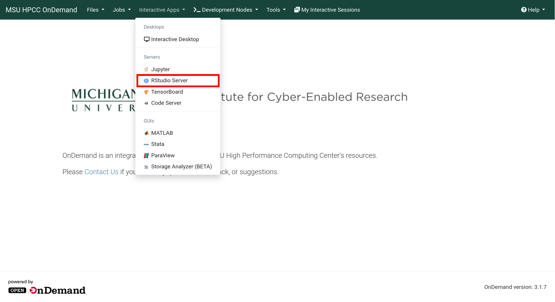
We’ll begin by logging in on OnDemand. Go to https://ondemand.hpcc.msu.edu. If you are prompted, choose Michigan State University as the Identity Provider, and log in using your MSU NetID and password. Before we get into any other OnDemand specifics, we’ll submit an RStudio job to get you up and running.
Go to the Interactive Apps tab and select RStudio Server.
RStudio Server vs RStudio
In ICER’s OnDemand interface, we use RStudio Server instead of just RStudio. This is a version of RStudio that runs on compute nodes and opens in your browser. Though it is possible to run plain RStudio on the HPCC, we use the Server version is as it displays more clearly and is easier to copy and paste into.
For the rest of this page, when we refer to “RStudio”, we really mean “RStudio Server”.
On the following screen you will be able to choose the options for your RStudio job. For this workshop, you should use the following options:
- R version: 4.3.2 (with additional CRAN packages, RECOMMENDED)
- Number of hours: 3
- Number of cores per task: 8
- Amount of memory: 5
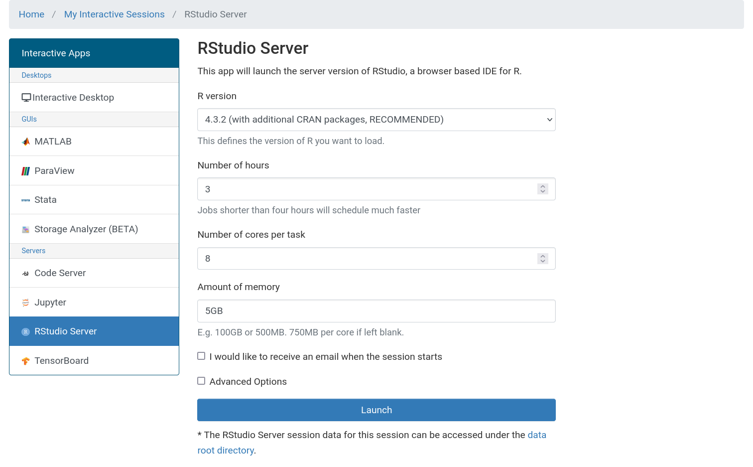
Additionally, click the Advanced Options checkbox and under Node type, select “amd20” (we’ll explain why later).
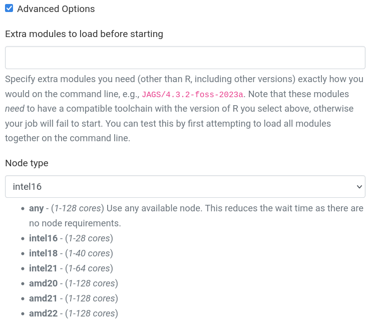
If you need to specify any other options (for example, if you want to run your session on a buy-in node and specify your SLURM account), you enter additional information in the Advanced Options section.
Select the Launch button and wait for your job to start. When your job is ready, you will see a card with all of the information for your job. The most important fields for now are the Host which is the node on the HPCC where you job is running and the Time Remaining which counts down from the requested number of hours.
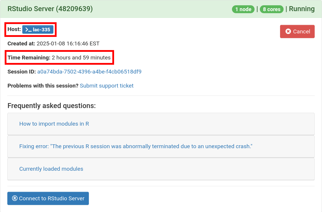
When you’re ready to access RStudio, you can click the Launch RStudio Server button. If you ever navigate away from this screen, you can always return to it by clicking the My Interactive Sessions button in the OnDemand navigation bar. On narrower screens, this button shrinks down to a graphic of a pair of overlapping cards next to the Tools dropdown.
RStudio
After Launching your RStudio session, a new tab in your browser will show an RStudio interface.
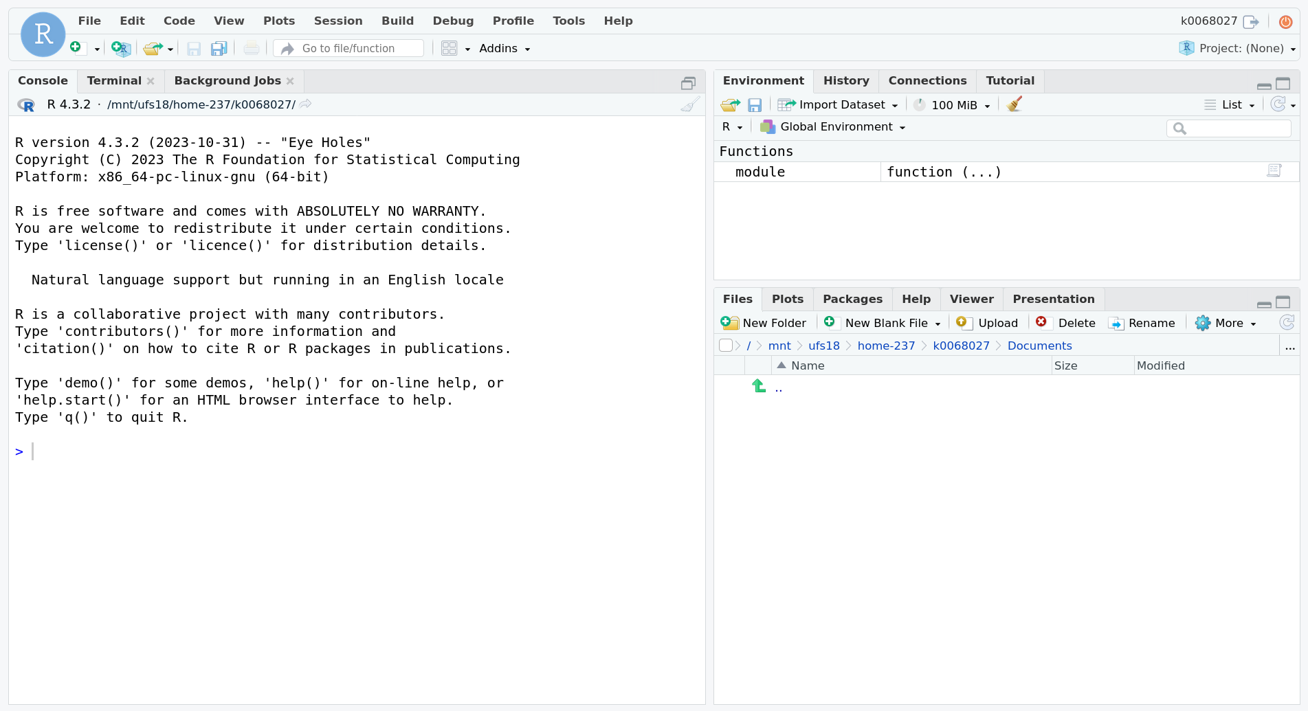
On startup, there are three main sections to RStudio: an R console, an environment section, and a file browser. Notice that the file browser starts in your HPCC home directory.
Open a file
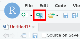
Use the RStudio interface to create a new R Script file.
Click the button that looks like a page with a plus sign right below the file menu and choose R Script.
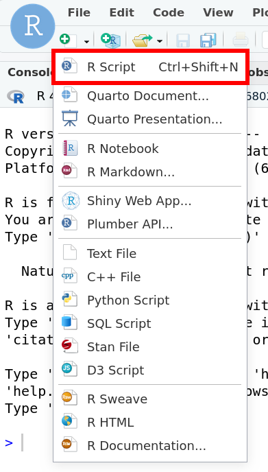
Notice that the R console shrinks to make room for the text editor.
Connect to your RStudio node from the command line
As discussed earlier, OnDemand tells you the Host that your RStudio job is running on. From time to time, you may need to run commands on this host from a command line. You have two options.
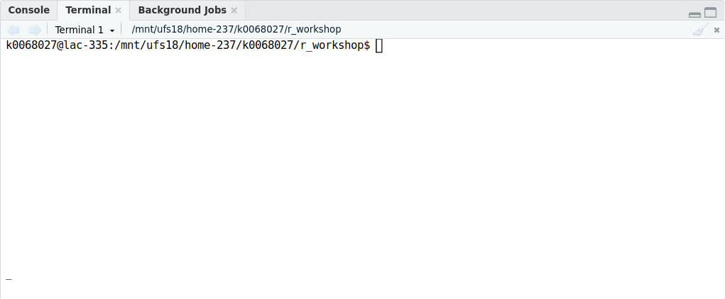
The RStudio terminal
Handily, RStudio provides a terminal for you to use! Right next to the R console, is a Terminal tab. Clicking this tab will start a terminal on the same node that RStudio is running on.
SSH
This can be accomplished through any terminal that you can SSH to the HPCC on. Since we’re already using OnDemand, we’ll use the built-in terminal.
Returning to the OnDemand window, open the Development Nodes dropdown from the navigation bar.
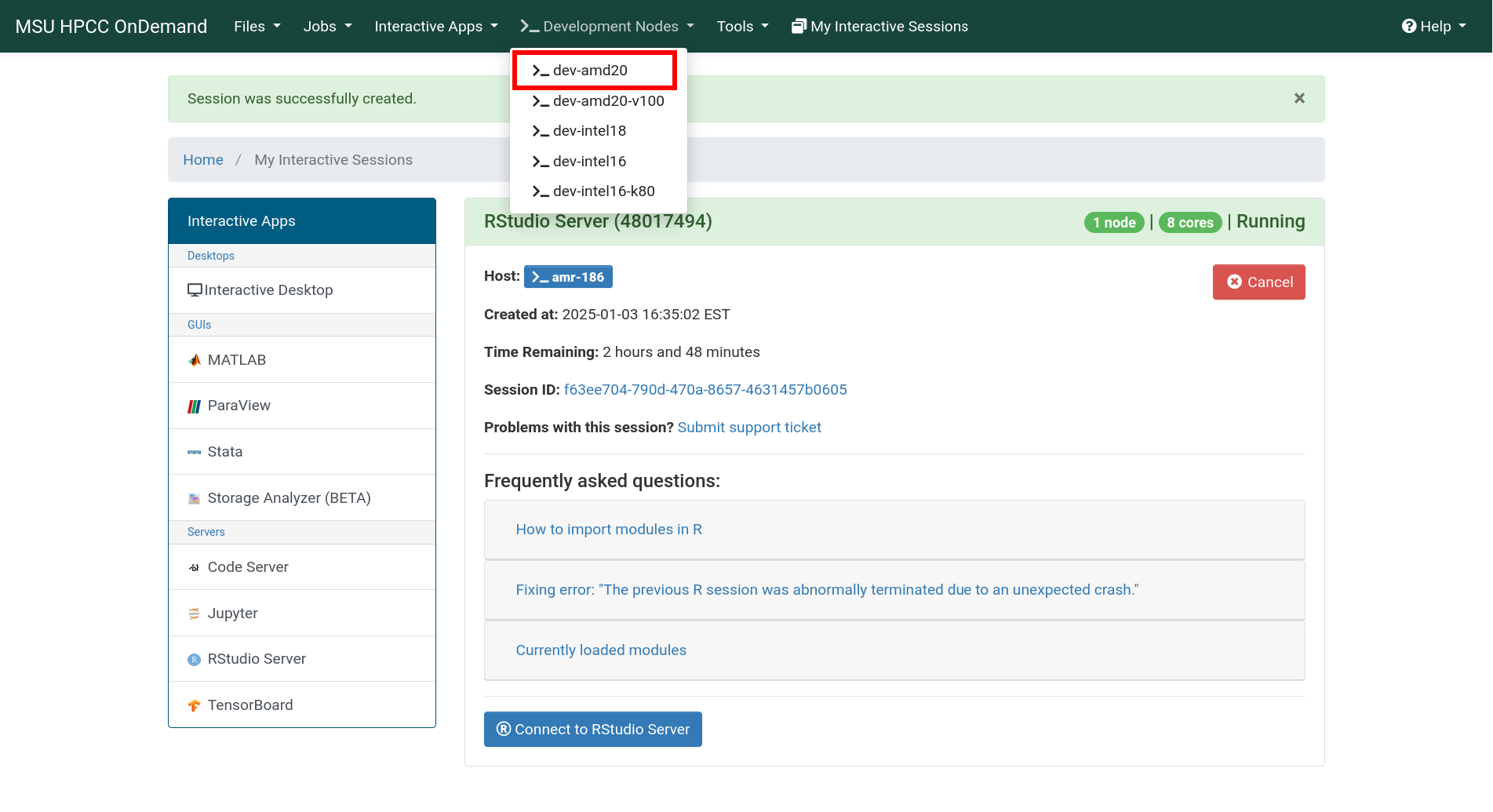
Choose the dev-amd20 development node, and a new tab
will open with a terminal there.
SSH outside of OnDemand
If you are not using an OnDemand terminal, you first need to manually
SSH into a development node. From your terminal (e.g., the built in
terminal on Mac or MobaXterm on Windows), SSH into the gateway via
ssh <netid>@hpcc.msu.edu, then SSH into a development
node, e.g., ssh dev-amd20.
Now find the Host your RStudio session is running on (remember, this information is always available in the My Interactive Jobs section in OnDemand), and in the development node terminal type
replacing <host> by the host your RStudio session
is running on.
Challenge
Run the top command via command line on the node your
RStudio session is running on and verify that indeed R is running
there.
Hint: If your node is busy, you can use
top -u <netid> (replacing <netid>
with your username) to see just your running processes.
Running top -u k0068027 (my username) from the RStudio
terminal shows the rsession command in the
COMMAND column representing the R session where we can
execute code. Scrolling through the entries, rserver (i.e.,
RStudio Server) also appears.
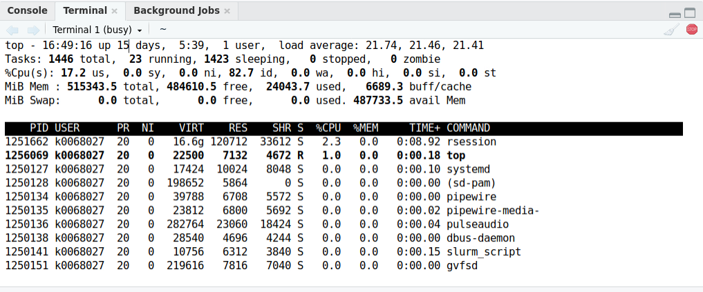
Depending on your screen width, you may have to use the arrow keys to
scroll to the right and see the COMMAND column.
- Start an RStudio Server session from OnDemand
- Access the command line of the node your process is running on through the RStudio terminal or SSH into the host OnDemand provides you.
Content from Managing R package installation and environment
Last updated on 2026-06-19 | Edit this page
Overview
Questions
- How can you install and organize packages in R?
- What are some best practices for setting up a project on the HPCC?
Objectives
- Explain where packages are kept and how to customize the location
- Demonstrate how to setup an RStudio project
- Share ways to effectively organize your projects for collaboration
Libraries
The HPCC has multiple versions of R installed, and many of those
versions have a large number of R packages pre-installed. But there will
come a time when your workflow requires a new package that isn’t already
installed. For this, you can use R’s built-in
install.packages() function.
Before we do that though, we should check which libraries we have
access to. We can do this by typing .libPaths() into the R
console:
R
.libPaths()
OUTPUT
[1] "/mnt/ufs18/home-237/k0068027/R/x86_64-pc-linux-gnu-library/4.3"
[2] "/cvmfs/ubuntu_2204.icer.msu.edu/2023.06/x86_64/generic/software/R-bundle-CRAN/2023.12-foss-2023a"
[3] "/cvmfs/ubuntu_2204.icer.msu.edu/2023.06/x86_64/amd/zen2/software/R/4.3.2-gfbf-2023a/lib/R/library"
We see three directories. The first is created for you in your home
directory. The third (or one like it, starting with
/cvmfs/ubuntu_2204.icer.msu.edu or
/opt/software-current) points to all of the packages that
are pre-installed with the base version of R. The second contains a
large set of additional packages from CRAN, forming a general base that
most users will be happy with.
When you use install.packages() in the future, by
default, it will install to the first entry in your
.libPaths().
One important point to note is that the library in your home
directory is labeled with 4.3 for version 4.3(.2) of R, the
default used by RStudio Server. If you ever use different versions of R,
it is important that the packages you use are consistent with those
versions. So, for example, if you choose to use R/4.2.2, you should make
sure that the library in your home directory returned by
.libPaths() ends in 3.2. Mixing versions will likely cause
your packages to stop working!
What’s the difference between a library and a package?
A library is just a collection of packages. When you use
library(<package>), you are telling R to look in your
libraries for the desired package. When you use
install.packages(<package>), you are telling R to
install the desired package into the first library on your
.libPaths().
What if you don’t have a user-writable library?
Sometimes, when starting R for the first time, it may happen that the
.libPaths() command won’t show you a library in your home
directory. Since the other library is shared by everyone on the HPCC,
you won’t be able to write to it.
Luckily, R knows this, and if you try to install a package, you will be offered to create a new user-writable library:
OUTPUT
Warning in install.packages :
  'lib = "/cvmfs/ubuntu_2204.icer.msu.edu/2023.06/x86_64/generic/software/R-bundle-CRAN/2023.12-foss-2023a"' is not writable
Would you like to use a personal library instead? (yes/No/cancel)
Answer yes, and you will be good to go!
Installing packages
Now, let’s try to install a package:
R
install.packages("cowsay")
You may then be asked to select a CRAN mirror. This is the location
where the package is downloaded from. Usually, 65 (or
something close by depending on what’s available) is a good choice for
us because it’s from the University of Michigan (closer means faster
downloads).
R will download and install the package. We can now use it like we normally would! From the R console:
R
library(cowsay)
say("Hello world!")
OUTPUT
 --------------
< Hello world! >
 --------------
      \
       \

        ^__^
        (oo)\ ________
        (__)\         )\ /\
             ||------w|
|| ||Do your packages require external dependencies?
Often, packages will require some extra software to install, run, or both. Getting external dependencies lined up correctly can be a big challenge, especially on the HPCC. Here are some general tips:
- Read the documentation for the package you’re using and take note of any dependencies you need and their versions. This information is also included under SystemRequirements on a package’s CRAN page.
- Make sure that software is available before you try to install/use
the R package. This could involve:
- Loading it through the HPCC module system. When using RStudio in
OnDemand, you have two options:
- Click the “Advanced Options” checkbox when you start a new RStudio Server session. The first option will allow you to enter HPCC modules you’d like to load before RStudio starts.
- Use the
modulecommand in R, preloaded when you start RStudio. For example, you can runmodule("load JAGS")from the Console to have access to theJAGSsoftware. Otherwise, you can load these packages and use R through the command line.
- Installing it yourself in a way that R can find it.
- Loading it through the HPCC module system. When using RStudio in
OnDemand, you have two options:
- If a package’s setup instructions suggest something like
sudo apt-get ...orsudo dnf install ...under the Linux instructions, this is a sign that it needs external dependencies. These methods won’t work for installation on the HPCC; instead, look for and load HPCC modules with similar names. - Sometimes you’ll need to load more than one module, but they will have dependencies that conflict with each other (or even R itself!). In this case, contact the research consultants at ICER and we will do our best to help you out.
A note about node type
The HPCC consists of many different node types. When we started our OnDemand job, we chose to use only amd20 nodes.
When R installs a package, it customizes it to the specific node type it was installed on. So if you use the same library on different node types, the packages are not guaranteed to work properly, often resulting in an “Illegal instruction error” or RStudio crashing.
To get around this, we recommend using the same node type when you use R, either through OnDemand, in job scripts, or on development nodes.
We’ve already seen how to do this in OnDemand (using the dropdown in
the Advanced Options section). You can do this in job scripts by adding
the line #SBATCH --constraint=<nodetype> (which we
will see in a later
episode).
Alternatively, you can use the tools discussed in this section to manually manage different libraries for different node types, though it can be tricky to manage properly.
Managing your projects
Now that we know how to install and use external packages, let’s talk about managing your code. When you use R, it helps to organize your code into separate directories that you can think of as projects. As we’ll see later, running R out of this project directory can make your life a lot easier!
But when RStudio starts, your working directory is always set to your home directory.
R
getwd()
OUTPUT
"/mnt/ufs18/home-237/k0068027"RStudio has it’s own solution to this: RStudio Projects! Let’s create one to test this out. Find the button in RStudio that looks like a plus sign on top of a cube near the edit menu.
Start by creating an RStudio Project with button that looks like a plus sign on top of a cube near the Edit menu.
Select New Directory, then New Project from the options. Under
Directory name, use r_workshop, and make sure that it’s a
subdirectory of your home directory ~. We’ll leave the
other options alone for now, but note that RStudio will integrate nicely
into a workflow using git and GitHub! Click Create Project to
finish.
Your new RStudio Project will be loaded. This means a few things:
- A new session of R will be started in the project directory.
- This directory will be your new working directory (check
getwd()!). - The file browser has moved to this directory.
- A file called
r_workshop.Rprojhas been created. This file saves some options for how you edit your project in RStudio.
At any time, you can navigate to your project directory in the
RStudio file browser and click the .Rproj file to load up
this project or any other.
Configuring your projects
What if we wanted to make some changes to the way that R operates?
There are two files that we can create to help us do that:
.Rprofile and .Renviron.
First, let’s suppose that we want to make sure we use the University of Michigan CRAN mirror install our packages. The R commands
R
r <- getOption("repos")
r["CRAN"] <- "https://repo.miserver.it.umich.edu/cran/"
options(repos = r)
will take care of this for us. To make sure this runs every time we
start R, we’ll put it in the .Rprofile file.
Use RStudio to open a new Text File and type
R
local({
  r <- getOption("repos")
  r["CRAN"] <- "https://repo.miserver.it.umich.edu/cran/"
  options(repos = r)
})
The local part ensures that no output from code we write
is available to us in the R session: just the options get set. It’s good
practice to put any code you write in your .Rprofile in a
call to local to keep R from accidentally loading any large
objects which slows down startup.
Save this in your r_workshop directory as
.Rprofile (don’t forget the leading .). Any
time R starts, it will look for a .Rprofile file in the
current directory, and execute all of the code before doing anything
else. To make this take effect in RStudio, you can restart R by going to
the Session menu, and select Restart R. To check our work, run
R
options()$repos
OUTPUT
                                      CRAN
"https://repo.miserver.it.umich.edu/cran/"
Now suppose that this project we’re working on uses some very special
packages that we don’t want in the library in our home directory. The
right way to do this is with a package manager like renv.
But for example’s sake, we’ll create a quick approximation with the
R_LIBS_USER environment variable and the
.Renviron file.
The R_LIBS_USER environment variable can be set to a
directory that you want to use as a library instead of the default one
we saw before in your home directory. If we’re running R from the
command line (which we’ll talk about
later), we could export this variable in the command line before you
start R:
But not only would we have to do this every time we run R, this
process is also hidden away behind the scenes when we use RStudio from
OnDemand! There’s another option: the .Renviron file.
Before R starts up (no matter if it’s from the command line or Rstudio),
it will look at all the environment variables in this file and set
them.
In RStudio, open a new Text File and type
R_LIBS_USER="./library"Then save this file in your r_workshop directory with
the name .Renviron. Now, restart R using the Session menu,
and check your .libPaths() in the R console:
R
.libPaths()
OUTPUT
[1] "/mnt/ufs18/home-237/k0068027/r_workshop/library"
[2] "/cvmfs/ubuntu_2204.icer.msu.edu/2023.06/x86_64/generic/software/R-bundle-CRAN/2023.12-foss-2023a"
[3] "/cvmfs/ubuntu_2204.icer.msu.edu/2023.06/x86_64/amd/zen2/software/R/4.3.2-gfbf-2023a/lib/R/library"
Great! We can even check that we’ve isolated ourselves from the
default home directory library by trying to load
cowsay:
R
library(cowsay)
Error in library(cowsay) : there is no package called 'cowsay'Other configuration locations
The .Rprofile and .Renviron files don’t
have to live in the directory you start R from. In fact, R checks for
them in a set order:
- In the directory where R is started.
- In your home directory.
- In a global directory where R is installed. On the HPCC, this is the
file
$R_HOME/etc/Renviron(you can check where$R_HOMEis withSys.getenv("$R_HOME")).
and uses the values in the first one it finds.
This means you can set a more global configuration by putting
environment variables and startup scripts in the .Renviron
and .Rprofile files in your home directory. However, if you
forget what defaults you setup there and you try to move to another
computer, you may have trouble running your code again. It’s best to use
these home directory files sparingly to preserve portability.
Packages for later
Install the following packages in your r_workshop
project library:
futuredoFutureforeachfuture.batchtools
Check to make sure these install into the right library.
Double checking our library paths
R
.libPaths()
OUTPUT
[1] "/mnt/ufs18/home-237/k0068027/r_workshop/library"
[2] "/cvmfs/ubuntu_2204.icer.msu.edu/2023.06/x86_64/generic/software/R-bundle-CRAN/2023.12-foss-2023a"
[3] "/cvmfs/ubuntu_2204.icer.msu.edu/2023.06/x86_64/amd/zen2/software/R/4.3.2-gfbf-2023a/lib/R/library"
we see that our r_workshop/library directory is
first.
If we install future, it goes into this directory:
R
install.packages("future")
OUTPUT
Installing package into `/mnt/ufs18/home-237/k0068027/r_workshop/library`
(as `lib` is unspecified)
A quick way to see which packages are installed in which library is to run
R
lapply(.libPaths(), list.files)
Startup and shutdown code
The functions .First and .Last (that don’t
take any arguments) can be defined in the .Rprofile file to
run any code before starting and after ending an R session respectively.
Define these functions so that R will print
### Hello <user> ### at the beginning of an R session
and ### Goodbye <user> ### at the end (where
<user> is your username).
Restart your R session to test your solution.
As a bonus, use Sys.getenv and the USER
environment variable to say hello and goodbye to whoever is using the
.Rprofile.
Note that since we are setting variables that we want to keep in our
session, the following lines should not be included in the
local block in the .Rprofile file.
R
.First <- function() cat("### Hello", Sys.getenv("USER"), "###\n")
.Last <- function() cat("### Goodbye", Sys.getenv("USER"), "###\n")
Best practices for a portable project (and when and how to break the rules)
It is very likely that you are not the only person working with your code: there are other people in your lab or outside that you should be ready to share your analyses with. There are a few ways to setup your R project to make things less painful to share.
And even if you’re not collaborating, you’re still sharing with future you! Staying organized will help you return to an old project and get up and running faster.
Tips:
- Don’t leave
install.packagescommands in your scripts. Run them from the R console, and document what you need so that others can install them themselves later. Or better yet, get a package isolation solution to do it for you, as discussed above. - Organize the files in your project into separate folders. A commonly
used setup is something like
-
data/for raw data that you shouldn’t ever change -
results/for generated files and output (e.g., you should be able to delete this folder and exactly regenerate it from your code.) -
src/for your code, like.Rfiles -
bin/for any other programs you need to run your analyses -
doc/for text documents associated with your project
-
- Use relative paths inside your project. Instead of using
C:\Users\me\Documents\lab_files\research\experiment1.csv, putexperiment1.csvinto thedata/directory in your project folder and only reference it asdata/experiment1.csv. - Reuse your code. If you need to run the same analysis on two
different inputs, don’t copy your script and find-and-replace
data/experiment1.csvwithdata/experiment2.csv. Instead, structure your script as a function that takes a filename as input. Then write a script that sources the script your function is in and calls that function with two different filenames. - Separate the steps in your analyses into separate scripts (which
ideally wrap the step into a function). You can chain all of your
scripts together in one
run_all.Rscript that sets up your input files and runs each step on those inputs in order.
All of this being said, rules of thumb can always be broken, but you should have a really good reason to do so. Oftentimes, using a supercomputer can be that reason.
For example, you may be using the HPCC to analyze some very large
files that wouldn’t be easy to share in a data/ directory
under your project. Maybe these live in your group’s research space on
the HPCC so you don’t have to copy them around. In this case, it might
make sense to use an absolute path to this file in your R scripts, e.g.,
/mnt/research/my_lab/big_experiment/experiment1.csv.
If you do decide to do this however, make sure you only do it one
time! This is a great use for the .Renviron file. Instead
of directly typing /mnt/research/my_lab/big_experiment/
into your code, set this as an environment variable in your
.Renviron:
When you need to access this directory from R, use
Sys.getenv():
R
data_dir <- Sys.getenv("DATA_DIR")
data <- read.csv(file.path(data_dir, "experiment1.csv"))
If somebody else wants to use your project outside of the HPCC and
downloads the data on their own, they just have to set the
DATA_DIR variable in the .Renviron file once
and for all. This can be a great place to keep user specific
configurations like usernames, secrets, or API keys.
- The
.libPaths()function shows you where R looks for and installs packages - Use the
.Renvironfile to set environment variables you’d like to use for your project - Add functions and set options in the
.Rprofilefile to customize your R session - Start R from your project directory and use relative paths
Content from Parallelizing your R code with future
Last updated on 2026-06-19 | Edit this page
Overview
Questions
- How can you use HPCC resources to make your R code run faster?
Objectives
- Introduce the R package
future - Demonstrate some simple ways to parallelize your code with
foreachandfuture_lapply - Explain different parallelization backends
Basics of parallelization
The HPCC is made up of lots of computers that have processors with lots of cores. Your laptop probably has a processor with 4-8 cores while the largest nodes on the HPCC have 192 cores.
All this said though, HPCC nodes are not inherently faster than standard computers. In fact, having many cores in a processor usually comes at the cost of slightly slower processing speeds. One of the primary benefits of running on the HPCC is that that you can speed up your throughput by doing many tasks at the same time on multiple processors, nodes, or both. This is called running your code in parallel.
Except for a few exceptions (like linear algebra routines), this speedup isn’t automatic! You will need to make some changes to your code so it knows what resources to use and how to split up its execution across those resources. We’ll use the “Futureverse” of R packages to help us do this quickly.
Writing code that runs on multiple cores
Let’s start with a small example of some code that can be sped up by running in parallel. In RStudio, create a new R Script and enter the following code:
R
t <- proc.time()

x <- 1:10
z <- rep(NA, length(x))  # Preallocate the result vector

for(i in seq_along(x)) {
  Sys.sleep(0.5)
  z[i] <- sqrt(x[i])
}

print(proc.time() - t)
Create a new directory in your r_workshop project called
src and save it as src/test_sqrt.R. Click the
Source button at the top of the editor window in RStudio, and see the
output:
OUTPUT
   user  system elapsed
  0.016   0.009   5.006
This means that it took about 5 seconds for the code to run. Of course, this all came from us asking the code to sleep for half a second each loop iteration! This is just to simulate a long running chunk of code that we might want to parallelize.
A digression on vectorization
Ignoring the Sys.sleep(0.5) part of our loop, if we just
wanted the square root of all of the elements in x, we
should never use a loop! R thrives with vectorization, meaning that we
can apply a function to a whole vector at once. This will also trigger
some of those linear algebra libraries that can auto-parallelize parts
of your code.
For example, compare
R
t <- proc.time()

x <- 1:10
z <- rep(NA, length(x))  # Preallocate the result vector
for(i in seq_along(x)) {
  z[i] <- sqrt(x[i])
}

print(proc.time() - t)
OUTPUT
   user  system elapsed
  0.004   0.000   0.005
to
R
t <- proc.time()

x <- 1:10
z <- sqrt(x)

print(proc.time() - t)
OUTPUT
   user  system elapsed
      0       0       0
Not only is the vectorized code much cleaner, it’s much faster too!
Let’s parallelize this with a combination of the foreach
and the doFuture packages. Start a new R script with the
following lines
R
library(foreach)
library(doFuture)
plan(sequential)

t <- proc.time()

x <- 1:10
z <- foreach(xi = x) %dofuture% {
  Sys.sleep(0.5)
  sqrt(xi)
}

print(proc.time() - t)
and save as src/test_sqrt_multisession.R.
Notice that this is very close to our original code, but we made a few changes:
- We changed the
forloop into aforeachstatement.- The
xi = xlets us iterate overxand usexias an element rather than indexing. - The block that happens on each “iteration” is preceded by
%dofuture%. This tellsforeachhow to run each of the iterations, and in this case, uses thefuturepackage behind the scenes.
- The
-
zis now the output offoreachstatement rather than preallocated and subsequently changed on each iteration of theforloop. Each element is the last result of the code block for each inputxi.
Let’s run the code:
OUTPUT
   user  system elapsed
  0.050   0.012   5.051
Huh? It’s slower! Well, we forgot one thing. We changed our code to get ready for parallelization, but we didn’t say how we want to parallelize it.
Well, actually, we did. The plan(sequential) line tells
future that we want to run each loop iteration
sequentially, i.e., the same exact way the original for loop works! We
just added some extra overhead of having the future package
manage it for us.
The multisession backend
To parallelize things, we change the plan. There are a few options,
but we’ll start with the multisession plan. Change
plan(sequential) to plan(multisession) and run
again:
OUTPUT
   user  system elapsed
  0.646   0.019   2.642
Much better! What future did behind the scenes is check how many cores we have allotted to our RStudio session with
R
availableCores()
OUTPUT
cgroups.cpuset
             8
and make that many R sessions in the background. Each of these sessions gets a loop iteration to run, and when finished, if there are still more, it will run another one.
We can tell future to use a certain number of workers in
the plan, which will override the number of cores. Add the
workers option to plan(multisession) like
R
plan(multisession, workers = 5)
and rerun to get
OUTPUT
   user  system elapsed
  0.327   0.010   1.923
It’s even faster! With five workers, each worker has exactly two iterations to work on, and we don’t have the overhead of the three extra ones that wait around to do nothing.
The multicore backend
In addition to a multisession plan, we can use the
multicore plan to utilize all of our cores. Instead of
starting multiple R sessions, future forks the main process
into as many processes as specified workers. This generally has less
overhead, and one major advantage is that all of the workers share the
memory of the original process. In the multisession plan,
each worker copied the part of x it had to work on into new
memory which can really add up for large inputs. However, in the
multicore case, since the memory is shared, it is not
writable.
Unfortunately, the multicore plan is less stable in GUI
environments like RStudio. Thus, it can only be used in scripts running from the command line, so we will
ignore it for now.
Writing code that runs on multiple nodes
Now that we know how to make the most of the cores we reserved, how
can we scale up further? One of the major benefits of the HPCC is the
fact that there are plenty of different nodes for you to run your code
on! With just a few changes to the future setup, we can
transition from a “multicore” to “multinode” setup.
The cluster backend
To use the cluster backend, you need a list of nodes you
can access through SSH. Usually, you would submit a SLURM job requesting
multiple nodes and use these, but we will save that for a future section.
For now, we’ll practice by using some development nodes.
Copy src/test_sqrt_multisession.R to
src/test_sqrt_cluster.R, and replace the plan
line with the following:
R
hostnames <- c("dev-amd20", "dev-amd20-v100")
plan(cluster, workers = hostnames)
When we run the code, we get:
OUTPUT
/opt/software-current/2023.06/x86_64/amd/zen2/software/R/4.3.2-gfbf-2023a/lib64/R/bin/exec/R: error while loading shared libraries: libicuuc.so.73: cannot open shared object file: No such file or directoryHmm, something went wrong. It turns out that future
isn’t always sure how to set up R on the hosts we pass it to build the
cluster with. We have to tell it how to start R, as well as some other
details, like what library path to use, and that it should set the
working directory on each node to our current working directory.
Start by creating a new bash script with the following information:
and save it as rscript.sh in the src
directory. This set of cryptic commands will become more clear in the
following sections. Then, from a command line, make it executable
with
Finally, we are ready to improve our plan setup:
R
hostnames <- c("dev-amd20", "dev-amd20-v100")
wd <- getwd()
rscript_cmd <- file.path(wd, "src", "rscript.sh")
setwd_cmd <- paste0("setwd('", wd, "')")
plan(cluster, workers = hostnames,
     rscript = rscript_cmd,
     rscript_libs = .libPaths(),
     rscript_startup = setwd_cmd)
Now let’s run again:
OUTPUT
user  system elapsed
  0.233   0.044   2.769
There was much more time setting up, but we were still able to save some time in the part that we measured!
The batchtools_slurm backend
As we saw, using cluster plan can be tricky to get
right. A much easier way to advantage of multiple nodes is to use the
batchtools.slurm backend. This allows us to submit SLURM
jobs for each iteration of our for loop. The HPCC scheduler will then
control where and when these jobs run, rather than you needing to
provide that information ahead of time.
The simplest way to do this, is to use the
future.batchtools package. Copy
src/test_sqrt_multisession.R to
src/test_sqrt_slurm.R, load the
future.batchtools package, and replace the
plan section with the batchtools_slurm
plan:
R
library(foreach)
library(doFuture)
library(future.batchtools)
plan(batchtools_slurm)
Running the code gives us
OUTPUT
   user  system elapsed
  6.916   2.083  39.614
So we experience a much longer wait… But this make sense! We just sent off ten SLURM jobs to sit in the HPCC queue, get started, do a tiny computation, shut down, and send back the result.
This is definitely not the kind of setting where we should
use the batchtools_slurm backend, but imagine if the inside
of the for loop was extremely resource intensive. In this case, it might
make sense to send each iteration off into its own job with its own
reserved resources.
Speaking of which, what resources did we ask for in each of these
submitted jobs? We never specified anything. The
future.batchtools package comes with a set of default
templates. Here’s the slurm.tmpl file in the
library/future.batchtools/templates directory under our
project directory:
BASH
#!/bin/bash
######################################################################
# A batchtools launch script template for Slurm
#
# Author: Henrik Bengtsson
######################################################################

#SBATCH --job-name=<%= job.name %>
#SBATCH --output=<%= log.file %>
#SBATCH --nodes=1
#SBATCH --time=00:05:00

## Resources needed:
<% if (length(resources) > 0) {
  opts <- unlist(resources, use.names = TRUE)
  opts <- sprintf("--%s=%s", names(opts), opts)
  opts <- paste(opts, collapse = " ") %>
#SBATCH <%= opts %>
<% } %>

## Launch R and evaluated the batchtools R job
Rscript -e 'batchtools::doJobCollection("<%= uri %>")'
Now, there are some parts that don’t look like like a normal SLURM script, but we see that each SLURM job automatically requests one node and five minutes. The remaining resources are set to the default values (usually 1 CPU and 750MB of memory).
What if you want to change these values? The strange lines in the
template SLURM script allow us to pass in extra resources when we set
the plan. For example, if you need each loop iteration to
have 1GB of memory and 10 minutes of runtime, we can replace the
batchtools_slurm line with
R
plan(batchtools_slurm, resources = list(mem = "1GB",
                                        time="00:10:00"))
The resources argument is a list where each entry’s name
is the SLURM constraint and the value is a string with the desired
value. See the list of job
specifications in the ICER documentation for more details.
Unfortunately, this method of specifying resources is not very
flexible. In particular, the resource names have to satisfy R’s variable
naming rules, which means that specifying cpus-per-task is
impossible because of the dashes.
Alternatively, it is better to create your own template script that
will be used to submit your jobs. If you save a template like the one
above to your working directory as batchtools.slurm.tmpl,
it will be used instead. For more information, see the future.batchtools
documentation.
Other ways to use the future backends
We decided to setup our parallelization in a for loop using the
foreach package. But there are a few other ways to do this
as well. Most fit the paradigm of defining a function to “map” over the
elements in an array.
One common example is using the lapply function in base
R. We could rewrite our example above using lapply (without
any parallelization) like this:
R
slow_sqrt <- function(x) {
  Sys.sleep(0.5)
  sqrt(x)
}

x <- 1:10
z <- lapply(x, slow_sqrt)  # apply slow_sqrt to each element of x
To parallelize, we can use the future.apply package,
replace lapply with future_lapply, and setup
the backend exactly the same way:
R
library(future.apply)
plan(multisession, workers = 5)

slow_sqrt <- function(x) {
  Sys.sleep(0.5)
  sqrt(x)
}

x <- 1:10
z <- future_lapply(x, slow_sqrt)
The “Futureverse” (i.e.,
the list of packages related to future) also includes
furrr, a future-ized version of the Tidyverse
package purrr. Additionally, the doFuture
package contains adapters to parallelize plyr and
BiocParallel mapping functions.
The upshot is that if you have code that’s setup (or can be setup) in
the style of mapping a function over arrays, you can parallelize it by
employing an adapter to the future backend.
- Setup code you want to parallelize as “mapping” a function over an array
- Setup a
futurebackend to distribute each of these function applications over cores, nodes, or both - Use the
batchtools_slurmbackend to havefuturesubmit SLURM jobs for you - Use a
futureadapter to link your code to the backend
Content from Using R on the command line
Last updated on 2026-06-19 | Edit this page
Overview
Questions
- How do you run R on the HPCC through the command line?
- How can I create plots when I’m not using a graphical interface?
Objectives
- Demonstrate how to find and load a desired version of R using the module system
- Demonstrate how to start an R console
- Demonstrate how to run R scripts with the
RScriptcommand
Accessing the HPCC through the terminal
Up to now, we’ve been using RStudio through OnDemand to write and run R code on the HPCC. Now, we’ll do the same things we’ve been doing, but solely through the command line. This will allow us to eventually submit SLURM batch scripts to run our code on compute nodes.
For now, we’ll start by running everything on a development node. Using our previous instructions to SSH into a development node, we can get a command line running on a development node. As a reminder, from a personal terminal, this looks something like
Make sure to use dev-amd20 since it matches
the node type we used in OnDemand.
Loading R
The command to run an R console from the command line is just
R!
OUTPUT
R version 4.3.2 (2023-10-31) -- "Eye Holes"
Copyright (C) 2023 The R Foundation for Statistical Computing
Platform: x86_64-pc-linux-gnu (64-bit)

R is free software and comes with ABSOLUTELY NO WARRANTY.
You are welcome to redistribute it under certain conditions.
Type 'license()' or 'licence()' for distribution details.

  Natural language support but running in an English locale

R is a collaborative project with many contributors.
Type 'contributors()' for more information and
'citation()' on how to cite R or R packages in publications.

Type 'demo()' for some demos, 'help()' for on-line help, or
'help.start()' for an HTML browser interface to help.
Type 'q()' to quit R.

>
This started up R version 4.3.2 with no problems, but there’s more
going on behind the scenes. In particular, by default, this version will
not have access to many additional packages pre-installed on the HPCC
(run .libPaths() or
lapply(.libPaths(), list.files) to check).
The HPCC packages up all of its available software into modules so that not every piece of software is available to everyone all of the time. To get access to R, we have to load its module.
Let’s first start by finding the version we’re interested in. We’ll
use the module spider command which searches through all
the modules for the ones we want:
OUTPUT
----------------------------------------------------------------------------
  R:
----------------------------------------------------------------------------
    Description:
      R is a free software environment for statistical computing and
      graphics.

     Versions:
        R/3.6.3-foss-2022b
        R/4.2.2-foss-2022b
        R/4.3.2-gfbf-2023a-ICER
        R/4.3.2-gfbf-2023a
        R/4.3.3-gfbf-2023b
        R/4.4.1-gfbf-2023b
        R/4.4.2-gfbf-2024a
        R/4.5.1-gfbf-2025a
     Other possible modules matches:
        ADMIXTURE  AOFlagger  APR  APR-util  Amber  Armadillo  Arrow  ...
...
We’ve abbreviated the output, but we can see that there are lots of different versions of R available! But note that none of these mention anything about extra packages like the versions in OnDemand do.
These are the base versions of R. To get access to more R packages that build on these base versions, you need to look for bundles:
OUTPUT
----------------------------------------------------------------------------
  R-bundle-Bioconductor:
----------------------------------------------------------------------------
    Description:
      Bioconductor provides tools for the analysis and coprehension of
      high-throughput genomic data.

     Versions:
        R-bundle-Bioconductor/3.16-foss-2022b-R-4.2.2
        R-bundle-Bioconductor/3.18-foss-2023a-R-4.3.2

----------------------------------------------------------------------------

...

----------------------------------------------------------------------------
  R-bundle-CRAN:
----------------------------------------------------------------------------
    Description:
      Bundle of R packages from CRAN

     Versions:
        R-bundle-CRAN/2023.12-foss-2023a
        R-bundle-CRAN/2024.06-foss-2023b
        R-bundle-CRAN/2024.11-foss-2024a
        R-bundle-CRAN/2025.10-foss-2025a

----------------------------------------------------------------------------
...
Note that the bundles are versioned differently (by year instead of R version). The best way to see which version of R is included is to load one and run R.
OUTPUT
R version 4.3.2 (2023-10-31) -- "Eye Holes"
Copyright (C) 2023 The R Foundation for Statistical Computing
Platform: x86_64-pc-linux-gnu (64-bit)

R is free software and comes with ABSOLUTELY NO WARRANTY.
You are welcome to redistribute it under certain conditions.
Type 'license()' or 'licence()' for distribution details.

  Natural language support but running in an English locale

R is a collaborative project with many contributors.


Type 'contributors()' for more information and
'citation()' on how to cite R or R packages in publications.

Type 'demo()' for some demos, 'help()' for on-line help, or
'help.start()' for an HTML browser interface to help.
Type 'q()' to quit R.

>
Great! This matches the exact R module that RStudio was using in OnDemand.
We now have an R console where we can run short lines of code, just
like from RStudio. As the output from R shows, type
q() to quit and return back to the command line.
If you’re asked to save the workspace image, it’s best practice to
say no since this can lead to long load times and less reproducible
sessions in the future. In fact, you can use the --vanilla
option when starting R to ensure it ignores things like your
.Renviron and .Rprofile changes. We will use
this option below to make sure we run our code in the cleanest
environment possible.
Loading external dependencies
As
mentioned when we were installing packages, sometimes R packages
need external dependencies to install and run. When you load the R
module using the module load commands above (before you
actually run R), this is also the time to load those
external dependencies.
Note that these dependencies and R will all need to be be compatible (e.g., use the same version of GCC and MPI). For example, a Bayesian modeling workflow might require the use of JAGS as dependencies for R packages. After loading R and its dependencies with
you can try loading a compatible JAGS module without specifying a version:
Then check which version gets loaded:
OUTPUT
Currently Loaded Modules:
1) GCCcore/12.3.0
2) zlib/1.2.13-GCCcore-12.3.0
...
127) R-bundle-CRAN/2023.12-foss-2023a
128) JAGS/4.3.2-foss-2023aIf this version will work, then great! If not, then you might try using a different version of R. Usually, newer versions of dependencies for popular R packages get installed with newer versions of R.
For more on finding and loading modules, checkout ICER’s module documentation.
Running one-liners and scripts with RScript
The R console is great for interactive work. But sometimes we might
want to just send some code to R to run and give us back the answer. For
this, we use the Rscript command.
First, let’s start by sending Rscript a single command
using the -e flag (which stands for “expression”):
OUTPUT
[1] "Tue Jan 7 17:29:05 2025"We get the same output as if we had run date() in an R
console or in a script! Note that we have to wrap the expression we want
to run in single quotes.
We can run multiple expressions at once. For example, let’s get the quotient and remainder of 128 divided by 11:
OUTPUT
[1] 11
[1] 7The real power of Rscript comes into play when we have
an actual script to run! Let’s run our previous one.
Rscript takes the path to the script as argument. We’ll
first change directory to the location of our script so we don’t need to
specify the entire path name.
OUTPUT
user system elapsed
0.238 0.003 1.698This is the equivalent of clicking the Source button while we have a
R script open in RStudio, or running
source('~/r_workshop/src/test_sqrt_multisession.R') from an
R console. Notice that we didn’t use the --vanilla option
here. This ensures that we use the local library setup in the project
directory.
Writing scripts that take command line arguments
Often, you will want to be able to pass extra arguments to your
scripts when you run them from the command line. The simplest way is to
use the commandArgs function in R which lets us access all
of the command line arguments as a character vector.
From the command line, open a new R script called
src/command_args.R in a text editor of your choice. If you
aren’t familiar with any, a good option is nano.
Our script will print out all of our command line arguments:
R
args <- commandArgs(trailingOnly = TRUE)
nargs <- length(args)
for(i in 1:nargs) {
cat("Argument", i, ":", args[i], "\n")
}
It’s important to use the trailingOnly = TRUE option
with commandArgs so that we only get the arguments after
the name of the script.
If you’re using nano, after typing the above code, press
ctrl+o followed by enter to save, then
ctrl+x to exit.
We can now run our script through Rscript with some
arguments:
OUTPUT
Argument 1 : a
Argument 2 : b
Argument 3 : c For a more sophisticated way to handle command line arguments (including flags, automated usage messages, default options, and more), check out optparse.
Challenge
Write an Rscript one-liner to print the numbers from 1 to 10.
Challenge
Write an Rscript one-liner to display the help for the
function strtoi (press “q” to exit).
Challenge
Write an Rscript that takes an integer as a command line argument and prints the numbers from 1 to that integer.
R
args <- commandArgs(trailingOnly = TRUE)
n <- strtoi(args[1])
for(i in 1:n) {
print(i)
}
Challenge
Copy test_sqrt_multisession.R into a new R script and
modify it to take an integer as a command line argument. Use the command
line argument to set the number of iterations in the
foreach loop. Additionally, make sure that the script
handles the case when no command line argument is passed (you can choose
the desired behavior).
R
library(foreach)
library(doFuture)
plan(multisession, workers = 5)
args <- commandArgs(trailingOnly = TRUE)
num_runs = 10 # default to 10 runs
if (length(args) > 0) {
num_runs <- strtoi(args[1])
}
t <- proc.time()
x <- 1:num_runs
z <- foreach(xi = x) %dofuture% {
Sys.sleep(0.5)
sqrt(xi)
}
print(proc.time() - t)
Plotting with the command line
You may wonder how you might run a plot using the terminal interface? For most terminals, if you plot with the command line version of R, either nothing happens or there is an error message. It may work on some terminals, if X11 Linux graphical interface is installed and the terminal is an X11-capable (for example on MacOS is ‘Quartz’ is installed, a new windows will appear). However when running in ‘batch’ mode using the cluster (described in the next session), there is no interface at all.
There are the following techniques for handling plots when using R on the command line on HPCC
- split your code into computation and presentation sections: run computation section using CLI/Batch on HPC, and after the computation is complete, save the output to be read into visualization code that you run on a machine with a graphic user interface (like OnDemand’s RStudio or even your laptop)
- capture all output to a file using commands like
pdf() - as part of your script, create an RMarkdown file that includes plotting (or other output), and use the render command in Rmarkdown to PDF or other format to be review later
We’ll describe the method to capture output into a PDF here.
A sample script that uses popular ggplot2 plotting
library and the pdf function to capture plots looks like
this:
R
library(ggplot2)
plotfile = file.path('results', 'testplots.pdf')
pdf(plotfile)
ggplot(iris, aes(x = Petal.Length, y = Petal.Width, color = Species)) +
geom_point() +
labs(title = "Edgar Anderson's Iris Data")
dev.off()
Save this into a file called src/plot.R.
In order to run this code, we first have to create the results directory on the command line with
Then we can run the script with
For much more details about using this technique, see Chapter 14 Output for Presentation of Winston Chang’s R Graphics Cookbook
Once you run the script and save the PDFs, the next challenge is to view them because, again, the terminal does not have the GUI to view PDFs.
You could
- download the PDF to your computer from the terminal using OnDemand file browser (or the MobaXterm client’s file browser)
- open with the OnDemand’s RStudio.
Challenge
One of the challenges with running scripts repeatedly is that it will overwrite the plot file with the same name. Modify the plotting script above that accepts a command line parameter for the the name of the PDF file. BONUS: how would you handle the case where there was no command line argument sent?
R
library(ggplot2)
args <- commandArgs(trailingOnly = TRUE)
# check if there was at least 1 arg
if length(args) >= 1 {
# assume the arg is a PDF file name, and use that to capture plots
plotfile = args[1]
pdf(plotfile)
}
# if no argument is sent, PDF capture is not enabled and the plot will display
ggplot(iris, aes(x = Petal.Length, y = Petal.Width, color = Species)) +
geom_point() +
labs(title = "Edgar Anderson's Iris Data")
dev.off()- Use
module spider Rto see the available versions of R on the HPCC - Use
module spider R-bundleto see the available bundles (including extra R packages) on the HPCC - Use
module load ...to get access to the desired version of R (or a bundle) - Run
Rfrom the command line to start an interactive R console - Use the
--vanillaoption to ignore extra configuration files - Run
Rscriptto run an R script - Use
commandArgsto parse command line arguments in an R script - Use
pdf()to capture plotting into a PDF file
Content from Submitting R code to SLURM
Last updated on 2026-06-19 | Edit this page
Overview
Questions
- How do you write a SLURM submission script?
Objectives
- Explain the general structure of a SLURM script
- Explain how and why to request different resources with SLURM
- Give sample template SLURM scripts for submitting R code
SLURM scripts
Now that we understand how to parallelize R code and run it on the command line, let’s put it all together. We’ll write a SLURM script to submit our code to run on compute nodes on the HPCC.
We’ve already seen an example of
a SLURM script in the parallelization section, where
future was submitting SLURM jobs for us. However, if we
want to have more control, we’ll have to understand how to write these
ourselves.
The basic structure of a SLURM script can be split into three parts:
- The
#!/bin/bash --loginline - Resources specifications
- Code you want to run (as if you’re inputting it on the command line)
The #!/bin/bash --login line always needs to be there.
It just tells the system to run your code with bash, which
is what you’re using on the command line.
The second section is where we specify resources. This is done using lines in the form
The options let you specify things like
- The time you need to run your code, e.g.,
#SBATCH --time=01:05:30for 1 hour, 5 minutes, and 30 seconds - The number of cores you want to run your code on, e.g.,
#SBATCH --cpus-per-task=8for 8 cores - The number of nodes you need to run your code on, e.g.,
#SBATCH --nodes=2for 2 nodes - The amount of memory your code will need, e.g.,
#SBATCH --mem=10GBfor 10GB or--mem-per-cpu=750MBfor 750MB per core you ask for - The node type, e.g.,
#SBATCH --constraint=amd20to run your code only on amd20 nodes - The SLURM account you want to use (if you have a buy-in node), e.g.,
#SBATCH --account=my_buyinto activate the buy-in nodes associated to themy_buyinaccount
Finally, you will add your code below these #SBATCH.
This code is exactly what you would enter on the command line to run
your R scripts as we showed in the previous epsiode.
A SLURM script template
BASH
#!/bin/bash --login
#SBATCH --time=00:05:00 # 5 minutes
#SBATCH --cpus-per-task=1 # Use 1 core
#SBATCH --mem-per-cpu=500MB # Use 500MB of memory per core requested
#SBATCH --nodes=1 # Use 1 node
#SBATCH --constraint=amd20 # Use only amd20 nodes
# Load the R module
module purge
module load R-bundle-CRAN/2023.12-foss-2023a
# Get to our project directory
cd ~/r_workshop
# Run the script
Rscript src/test_sqrt.R
# Bonus: write information about our job in the output file
scontrol show job $SLURM_JOB_IDA template like this will work for you 90% of the time, where all you need to do is set your resources correctly, load the right version of R, set the directory you want to work in, and choose your script.
SLURM script submission
Create a new directory in our R project directory called
slurm, and save the above file there as
single_core.sh. Then submit the script with
sbatch:
The script will sit in the queue until its resources are available. We can check on its status with
After the script has run, we can see its output in a file with a name
like slurm-<jobid>.out in the current working
directory.
OUTPUT
   user  system elapsed
  0.027   0.010   5.042
JobId=48169646 JobName=single_core.R
   UserId=k0068027(2238) GroupId=math(2011) MCS_label=N/A
   Priority=59669 Nice=0 Account=general QOS=k0068027
   JobState=RUNNING Reason=None Dependency=(null)
   Requeue=1 Restarts=0 BatchFlag=1 Reboot=0 ExitCode=0:0
   RunTime=00:00:17 TimeLimit=00:05:00 TimeMin=N/A
   SubmitTime=2025-01-07T17:33:34 EligibleTime=2025-01-07T17:33:34
   AccrueTime=2025-01-07T17:33:34
   StartTime=2025-01-07T17:33:50 EndTime=2025-01-07T17:38:50 Deadline=N/A
   SuspendTime=None SecsPreSuspend=0 LastSchedEval=2025-01-07T17:33:50 Scheduler=Main
   Partition=general-short AllocNode:Sid=dev-amd20:1882606
   ReqNodeList=(null) ExcNodeList=(null)
   NodeList=amr-184
   BatchHost=amr-184
   NumNodes=1 NumCPUs=1 NumTasks=1 CPUs/Task=1 ReqB:S:C:T=0:0:*:*
   ReqTRES=cpu=1,mem=500M,node=1,billing=76
   AllocTRES=cpu=1,mem=500M,node=1,billing=76
   Socks/Node=* NtasksPerN:B:S:C=0:0:*:* CoreSpec=*
   MinCPUsNode=1 MinMemoryCPU=500M MinTmpDiskNode=0
   Features=[intel18|(amr|acm)|nvf|nal|nif|amd24] DelayBoot=00:00:00
   OverSubscribe=OK Contiguous=0 Licenses=(null) Network=(null)
   Command=/mnt/ufs18/home-237/k0068027/r_workshop/single_core.R
   WorkDir=/mnt/ufs18/home-237/k0068027/r_workshop
   Comment=stdout=/mnt/ufs18/home-237/k0068027/r_workshop/slurm-48169646.out
   StdErr=/mnt/ufs18/home-237/k0068027/r_workshop/slurm-48169646.out
   StdIn=/dev/null
   StdOut=/mnt/ufs18/home-237/k0068027/r_workshop/slurm-48169646.out
   TresPerTask=cpu=1
Congratulations! We’ve just completed the workflow for submitting any job on the HPCC.
Submitting a multicore job
Copy your submission script to slurm/multi_core.sh.
Adjust it to request five cores and change it so that you run a copy of
src/test_sqrt_multisession.R with a multicore
backend for future with five workers. Submit the job and
compare the time it took to run with the single core job.
slurm/multi_core.sh:
BASH
#!/bin/bash --login

#SBATCH --time=00:05:00  # 5 minutes
#SBATCH --cpus-per-task=5  # Use 5 cores
#SBATCH --mem-per-cpu=500MB  # Use 500MB of memory per core requested
#SBATCH --nodes=1  # Use 1 node
#SBATCH --constraint=amd20  # Use only amd20 nodes

# Load the R module
module purge
module load R-bundle-CRAN/2023.12-foss-2023a

# Get to our project directory
cd ~/r_workshop

# Run the script
Rscript src/test_sqrt_multicore.R

# Bonus: write information about our job in the output file
scontrol show job $SLURM_JOB_IDsrc/test_sqrt_multicore.R:
R
library(foreach)
library(doFuture)
plan(multicore, workers = 5)

t <- proc.time()

x <- 1:10
z <- foreach(xi = x) %dofuture% {
  Sys.sleep(0.5)
  sqrt(xi)
}

print(proc.time() - t)
Cleaning up the output
Leaving the output in the directory we run the script in will get messy. For the steps below, you will need the list of SLURM job specifications.
- Create the directory
resultsin your project directory. - For the previous job script, change the name for the job allocation
to
multicore-sqrt. - Change it so the output and error files are stored in your project
directory under
results/<jobname>-<jobid>.outandresults/<jobname>-<jobid>.errwhere<jobname>is the name you set in the previous step and<jobid>is the number that SLURM assigns your job.
Hint: you can reference the job ID in #SBATCH
lines with %j and the job name with %x.
multi_core.sh:
BASH
#!/bin/bash --login

#SBATCH --time=00:05:00  # 5 minutes
#SBATCH --cpus-per-task=5  # Use 5 cores
#SBATCH --mem-per-cpu=500MB  # Use 500MB of memory per core requested
#SBATCH --nodes=1  # Use 1 node
#SBATCH --constraint=amd20  # Use only amd20 nodes
#SBATCH --job-name=multicore
#SBATCH --output=~/r_workshop/results/%x-%j.out
#SBATCH --error=~/r_workshop/results/%x-%j.err

# Load the R module
module purge
module load R-bundle-CRAN/2023.12-foss-2023a

# Get to our project directory
cd ~/r_workshop

# Run the script
Rscript src/test_sqrt_multicore.R
Submitting SLURM scripts for code that runs on multiple nodes
Using the future package
In the section on writing parallel code across multiple nodes using
the future package, we discussed two approaches: using the
cluster backend, and having future submit
SLURM jobs for you. In the latter case, you would only need to submit
your controller script to SLURM using a simple submission script like
the one above. The batchtools_slurm backend will submit
SLURM jobs for the hard work that you want parallelized (though, as
discussed, you may need to write a template script).
In the former case of using the cluster backend, we had
to tell future which nodes we want it to run on. Luckily
future has SLURM in mind and can query the nodes available
in your SLURM job with
parallelly:availableWorkers(methods = "Slurm"). You can
then use these as the workers when specifying the plan
like
For MPI jobs
MPI is a one of the most popular ways to write code in many languages
that runs on multiple nodes. You may write something that uses it
explicitly (e.g., the Rmpi
or pdbMPI
packages), or implicitly, by using a package that uses MPI behind the
scenes (e.g., doMPI).
Any code using MPI must be called in a special way that lets the code
know about the environment it’s running on. Practically, this means that
you need to preface the Rscript command with
srun with the option --cpus-per-task so MPI
knows how many CPUs it can use per task.
Here is an example script:
BASH
#!/bin/bash --login

#SBATCH --time=00:10:00  # 10 minutes
#SBATCH --tasks=6  # MPI will start 6 versions of the program
#SBATCH --cpus-per-task=8  # Use 8 cores per task (48 in total)
#SBATCH --mem-per-cpu=1GB  # Use 1GB of memory per core requested
#SBATCH --nodes=2  # Distribute the tasks across 2 nodes
#SBATCH --constraint=amd20  # Use only amd20 nodes

# Load the R module
module purge
module load R-bundle-CRAN/2023.12-foss-2023a

# Get to our project directory
cd ~/r_workshop

# Run the script
srun --cpus-per-task=$SLURM_CPUS_PER_TASK Rscript src/some_MPI_script.R

# Bonus: write information about our job in the output file
scontrol show job $SLURM_JOB_ID
Notice that we added an #SBATCH line for
tasks and used the $SLURM_CPUS_PER_TASK
variable to set the option for srun. This ensures that
whatever we set in the #SBATCH --cpus-per-task line will be
used by srun.
- A SLURM script requests resources
- Generally, the only code you need in a SLURM script is loading the R
module, changing to the right directory and running your R code with
Rscript - Check the status of your jobs with
squeue --me